Spherical Harmonics
2. Spherical Harmonic Lighting
Spherical Harmonic Lighting: The Gritty Details
2.1 Computer Rendering Background
Computer Rendering Background. Render Equation - integral the ‘Diffuse surface reflection’ over a hemisphere.
- Monte Carlo Integration, based on Probability theory - sampling over the hemisphere.
- Orthogonal Basis Functions, using Associated Legendre Polynomials.
- use recurrence relations to generation the polynomials.
2.2. Spherical Harmonics
Real Spherical Harmonics (~ Fourier transform defined across the surface of a sphere).
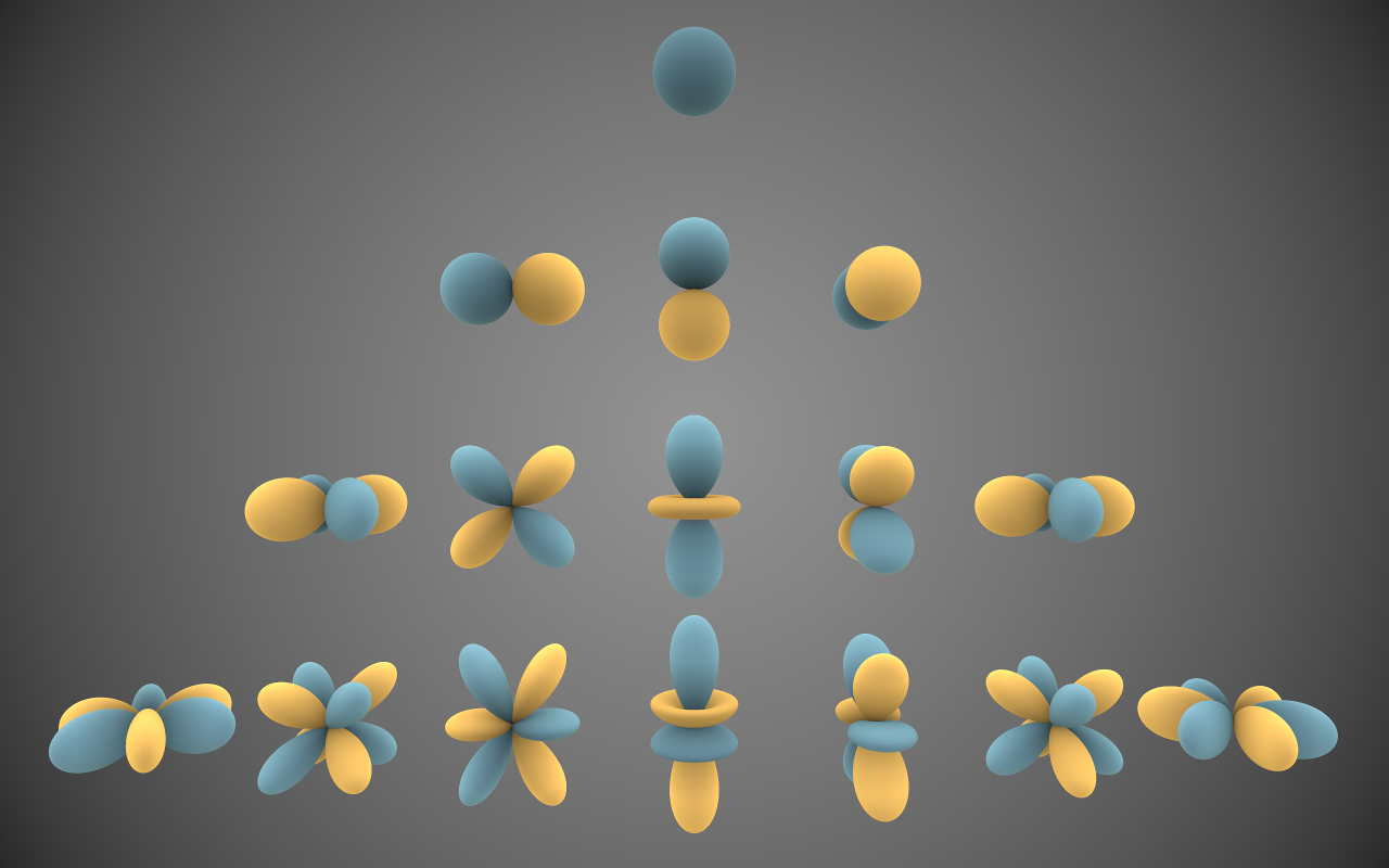
\[y_{l}^{m}(\theta, \varphi) = \begin{cases} \sqrt{2}K_{l}^{m} cos(m\varphi) P_{l}^{m}(cos\theta) \quad \quad m > 0\\ \sqrt{2}K_{l}^{m} sin(-m\varphi) P_{l}^{-m}(cos\theta) \quad \quad m < 0 \\ K_{l}^{0}P_{l}^{0}(cos\theta) \quad \quad m = 0 \end{cases} \quad \quad where \quad l \in \mathcal{R}^{+}, -l\le m\le l\] \[K_{l}^{m} = \sqrt{\frac{(2l + 1)}{4\pi} \frac{(l-|m|)!}{(l+|m|)!}}\]Visual representations of the first 4 bands of real spherical harmonic functions. Blue portions are regions where the function is positive, and yellow portions represent regions where it is negative.
Sampling to get light integral.
\[c_{i} = \frac{4\pi}{N}\sum_{j=1}^{N}light(x_{j})y_{i}(x_{j})\]Properties:
- Orthogonal & Orthonormal.
- Rotationally invariant.
- Signal Convolution - Adding transfer function is multiply-adds: \(\int_{S}L(s)t(s)ds = \sum_{i=0}^{n^{2}}L_{i}t_{i}\) (dot product of their coefficients).
- Signal Triple Product.
- Rotate SH projected function with block-diagonal matrix.